Hypothesis Testing
Introduction
Organization
- 15h of lectures, 18h of TD
- \(12^{th}\) may: Exam (2h)
- Lecture notes and slides on the website
- Wooclap sessions [Test]
Evaluation
- One final exam of 2h (QCM and paper exercise)
Objective
- Given a general decision problem
- Introduce precise notations to describe the pb
- formulate mathematically hypotheses \(H_0\) (a priori) and \(H_1\) (alternative)
- Choose a statistic adapted to the problem
- Compute this statistic and its pvalue (or an approx.)
- Conclude and make a decision
General Principles
- Fix an objective: test whether the drug lowers blood pressure
- Design an experiment: clinical trial comparing drug vs placebo
- Define hypotheses
- Null hypothesis \(H_0\): drug has no effect
- Alternative hypothesis \(H_1\): drug lowers blood pressure
- Define a decision rule: reject \(H_0\) if p-value < α (e.g., 5%)
- Collect Data: measure blood pressure change in both groups
- Apply the decision rule: reject \(H_0\) or not
- Draw a conclusion: should the drug be approved or run more trials?
What is a p-value?
p-value = probability of observing a result as extreme (or more) assuming \(H_0\) is true
Example: drug trial shows 8 mmHg blood pressure drop
- p-value = 0.03 means:
- → “If the drug had no effect, there’s only a 3% chance of seeing such a large drop by random chance alone”
Decision Rule
| p-value | Interpretation |
|---|---|
| p < 0.05 | Reject \(H_0\) → drug likely works |
| p ≥ 0.05 | Do not reject \(H_0\) → not enough evidence |
⚠️ A small p-value does not prove \(H_1\) is true — it only says \(H_0\) is unlikely given the data.
Good and Bad Decisions
| Decision | \(H_0\) True | \(H_1\) True |
|---|---|---|
| \(T=0\) | True Negative (TN) |
False Negative (FN)
|
| \(T=1\) |
False Positive (FP)
|
True Positive (TP) |
Dice Biased Toward 6
- Objective: test if Bob is cheating with a biased dice
- Experiment: Bob rolls the dice \(10\) times
- Hypotheses:
- \(H_0\): the probability of getting \(6\) is \(1/6\)
- \(H_1\): the probability of getting \(6\) is larger than \(1/6\)
- Decision rule: reject \(H_0\) if p-value \(< 0.05\)
- Data: the dice falls \(10\) times on \(6\)
- Decision: p-value \(= (1/6)^{10} \approx 10^{-8} < 0.05\) → reject \(H_0\)
- Conclusion: strong evidence Bob is cheating!
Fairness of Dice
- We observe \((X_1, \dots, X_n)\) iid where \(X_i \in \{1, \dots, 6\}\) with \(\mathbb{P}(X_i = k) = p_k\)

Fairness of Dice
⚠️ Same data, two conclusions
\(H_0: p_6 = 1/6\) vs \(H_1: p_6 > 1/6\)
Here: do not reject \(H_0\) (\(H_0\) is “likely”)
\(H_0:\) dice is fair vs \(H_1: \exists k: p_k > 1/6\)
Here: reject \(H_0\) (\(H_0\) is “unlikely”)
Medical Test
- Objective: test if a patient has high cholesterol
- Experiment: measure LDL cholesterol level (mg/dL)
- Hypotheses:
- \(H_0\): LDL cholesterol is normal \(\sim \mathcal{N}(100, 25)\)
- \(H_1\): LDL cholesterol is high
Medical Test
- Decision rule: reject if \(P_0(X \geq x_{obs}) \leq 0.05\)
- Collect data: \(x_{obs}=152\)
- Make a decision: calculate \(P_0(X \geq 152)=0.019\)
- Conclusion ?


Probability Basics
Recall of Proba: Continuous Measures
- PDF (Density): \(x \mapsto p(x)\) where \(\mathbb P(X\in[x,x+dx]) = p(x)dx\)
- CDF: \(x \mapsto \int_{-\infty}^x p(x')dx'\)
\(\alpha\)-quantile \(q_{\alpha}\): \(\int_{-\infty}^{q_{\alpha}} p(x)dx = \alpha\)
\(\Leftrightarrow \mathbb P(X \leq q_{\alpha}) = \alpha\)
Recall of Proba: Discrete Measures
Consider a probability measure \(P\) on \(\mathbb R\) with \(X \sim P\).
- PMF (Density): \(\mathbb P(X=x) = P(\{x\})=p(x)\)
- CDF: \(x \mapsto \sum_{x' \leq x} p(x')\)
\(\alpha\)-quantile \(q_{\alpha}\): \(\inf\{q \in \mathbb R:~\sum_{x_i \leq q}p(x_i) \geq \alpha\}\)
Example: Gaussian Distribution
Gaussian \(\mathcal N(\mu,\sigma)\): \[p(x) = \frac{1}{\sqrt{2\pi \sigma^2}}e^{-\frac{(x-\mu)^2}{2\sigma^2}}\]

Approximation of sum of iid RV (Central Limit Theorem)
Example: Gaussian Distribution
Gaussian \(\mathcal N(\mu,\sigma)\): \(p(x) = \frac{1}{\sqrt{2\pi \sigma^2}}e^{-\frac{(x-\mu)^2}{2\sigma^2}}\)
Approximation of sum of iid RV (CLT)
Example: Binomial Distribution
Binomial \(\mathrm{Bin}(n,q)\): \(p(x)= \binom{n}{x}q^x (1-q)^{n-x}\)

Number of successes among \(n\) Bernoulli \(q\)
Example: Exponential Distribution
Exponential \(\mathcal E(\lambda)\): \(p(x) = \lambda e^{-\lambda x}\)

Waiting time for an atomic clock of rate \(\lambda\)
Example: Geometric Distribution
Geometric \(\mathcal{G}(q)\): \(p(x)= q(1-q)^{x-1}\)

Index of first success for iid Bernoulli \(q\)
Example: Gamma Distribution
Gamma \(\Gamma(k, \lambda)\): \(p(x) = \frac{\lambda^k x^{k-1}e^{-\lambda x}}{(k-1)!}\)

Waiting time for \(k\) atomic clocks of rate \(\lambda\)
Example: Poisson Distribution
Poisson \(\mathcal{P}(\lambda)\): \(p(x)=\frac{\lambda^x}{x!}e^{-\lambda}\)

Number of ticks before time \(1\) of clock \(\lambda\)
Basics of Hypothesis Testing
Estimation VS Test
We observe some data \(X\) in a measurable space \((\mathcal X, \mathcal A)\).
Example: \(\mathcal X = \mathbb R^n\), \(X= (X_1, \dots, X_n)\).
Estimation
- One set of distributions \(\mathcal P\) parameterized by \(\Theta\) \[\mathcal P = \{P_{\theta},~ \theta \in \Theta\}\]
- \(\exists \theta \in \Theta\) such that \(X \sim P_{\theta}\)
Goal: estimate a function of \(P_{\theta}\), e.g. \(\int x \, dP_{\theta}\) or \(\int x^2 \, dP_{\theta}\)
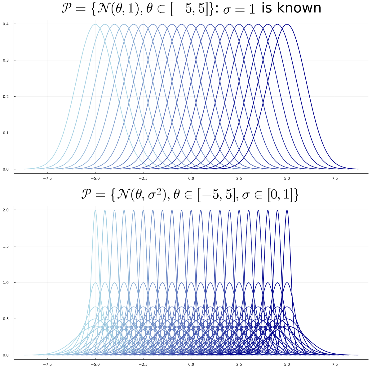
Test
- Two sets of distributions \(\mathcal P_0\), \(\mathcal P_1\) with disjoint \(\Theta_0\), \(\Theta_1\) \[\mathcal P_0 = \{P_{\theta} : \theta \in \Theta_0\}, ~~~~ \mathcal P_1 = \{P_{\theta} : \theta \in \Theta_1\}\]
- \(\exists \theta \in \Theta_0 \cup \Theta_1\) such that \(X \sim P_{\theta}\)
Goal: decide between \(H_0: \theta \in \Theta_0\) or \(H_1: \theta \in \Theta_1\)
Test Model
- Two sets of distributions \(\mathcal P_0\), \(\mathcal P_1\) with disjoint \(\Theta_0\), \(\Theta_1\) \[\mathcal P_0 = \{P_{\theta} : \theta \in \Theta_0\}, ~~~~ \mathcal P_1 = \{P_{\theta} : \theta \in \Theta_1\}\]
- \(\exists \theta \in \Theta_0 \cup \Theta_1\) such that \(X \sim P_{\theta}\)
Goal: decide between \(H_0: \theta \in \Theta_0\) or \(H_1: \theta \in \Theta_1\)
Types of Problems
- Simple VS Simple: \(\Theta_0 = \{\theta_0\}\) and \(\Theta_1 = \{\theta_1\}\)
- Simple VS Multiple: \(\Theta_0 = \{\theta_0\}\)
- Multiple VS Multiple: otherwise
Simple VS Simple

Multiple VS Multiple
Parametric VS Non-Parametric
- Parametric: \(\Theta_0\) and \(\Theta_1\) included in subspaces of finite dimension
- Non-parametric: otherwise
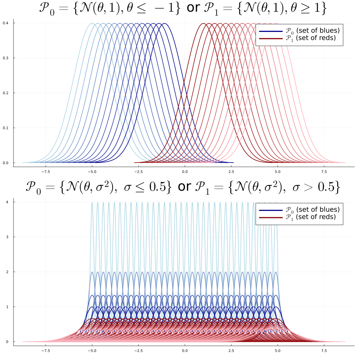
Example (Multiple VS Multiple Parametric):
- \(H_0: X \sim \mathcal N(\theta,\sigma)\), \(\theta < 0\), \(\sigma > 0\) → \(\Theta_0 \subset \mathbb R^2\)
- \(H_1: X \sim \mathcal N(\theta,\sigma)\), \(\theta > 0\), \(\sigma > 0\) → \(\Theta_1 \subset \mathbb R^2\)
Decision Rule
A Decision Rule or Test \(T\) is a measurable function: \[T : \mathcal X \to \{0,1\}\]
- It can depend on \(\mathcal P_0\) and \(\mathcal P_1\)
- but not on any unknown parameter
- \(T(x) = 0\) (or \(1\)) for all \(x\) is the trivial decision rule
Test Statistic
A Test Statistic \(\psi\) is a measurable function: \[\psi : \mathcal X \to \mathbb R\]
- It can depend on \(\mathcal P_0\) and \(\mathcal P_1\)
- but not on any unknown parameter
Rejection Region
For a test \(T\) with statistic \(\psi\), the rejection region \(\mathcal R \subset \mathbb R\) is: \[\mathcal R = \{\psi(x) \in \mathbb R:~ T(x)=1\}\]
→ Set of values of the statistic that lead to rejecting \(H_0\)
Critical Region
For a test \(T\), the critical region \(\mathcal C \subset \mathcal X\) is: \[\mathcal C = \{x \in \mathcal X:~ T(x)=1\}\]
→ Set of observations that lead to rejecting \(H_0\)
⚠️ These terms are sometimes used interchangeably, but we distinguish them in this course.
Example of Rejection Region
\[ \begin{aligned} T(x) &= \mathbf{1}\{\psi(x) > t\}:~~~~~~\mathcal R = (t,+\infty)\\ T(x) &= \mathbf{1}\{\psi(x) < t\}:~~~~~~\mathcal R = (-\infty,t)\\ T(x) &= \mathbf{1}\{|\psi(x)| > t\}:~~~~~~\mathcal R = (-\infty,t)\cup (t, +\infty)\\ T(x) &= \mathbf{1}\{\psi(x) \not \in [t_1, t_2]\}:~~~~~~\mathcal R = (-\infty,t_1)\cup (t_2, +\infty)\; \end{aligned} \]
Simple VS Simple
Simple VS Simple Problem
We observe \(X \in \mathcal X=\mathbb R^n\). We fix two known distributions \(P\) and \(Q\).
The problem:
\(H_0: X \sim P\) or \(H_1: X \sim Q\)
Warning
We know \(P\) and \(Q\) but not whether \(X \sim P\) or \(X \sim Q\)
Level and Power
Level and Power
Consider a simple VS simple problem. The Level of a test \(T\) is defined as
\[\alpha = P(T(X)=1) = P(X \in \mathcal C) \quad \text{(type-1 error)}\]
Its power is defined as
\[\beta = Q(T(X)=1) = Q(X \in \mathcal C)\]
\(1 - \beta\) is the type-2 error
Decision Table
| Decision | \(H_0: X \sim P\) | \(H_1: X \sim Q\) |
|---|---|---|
| \(T=0\) | ✓ \(1-\alpha\) | ✗ \(1-\beta\) |
| \(T=1\) | ✗ \(\alpha\) | ✓ \(\beta\) |
Unbiased: \(\beta \geq \alpha\)
\(\alpha = 0\) for trivial test \(T(x)=0\)… but \(\beta = 0\) too!
Likelihood Ratio Test
Consider the simple VS simple problem \(H_0\): \(X \sim P\) VS \(H_1\): \(X \sim Q\).
Question: which test \(T\) maximizes \(\beta\) at fixed \(\alpha\)?
Likelihood ratio statistic
\[\psi(x)=\frac{dQ}{dP}(x) = \frac{q(x)}{p(x)}\]
Likelihood ratio test
\[T^*(x)=\mathbf 1\left\{\frac{q(x)}{p(x)} > t_{\alpha}\right\}\]
where \(t_{\alpha}\) is the \(\alpha\)-quantile: \[\mathbb P_{X \sim P}\left(\frac{q(X)}{p(X)} > t_{\alpha}\right) = \alpha\]
Neyman-Pearson’s Theorem
Neyman-Pearson’s Theorem
The Likelihood Ratio Test of level \(\alpha\) maximizes the power among all tests of level \(\alpha\).
Recall: \(T^*(x)=\mathbf 1\left\{\frac{q(x)}{p(x)} > t_{\alpha}\right\}\) where \(P(T^*(X)=1) = \alpha\)
Equivalent to Log-Likelihood Ratio Test:
\[T^*(x)=\mathbf 1\left\{\log\left(\frac{q(x)}{p(x)}\right) > \log(t_{\alpha})\right\}\]
Neyman-Pearson: Proof Sketch
Let \(T\) be any test with level \(\alpha\). We want to show \(\beta^* \geq \beta\).
\[\beta^* - \beta = Q(T^*=1) - Q(T=1) = \int (T^* - T) dQ\]
\[= \int (T^* - T) \frac{q}{p} dP\]
Proof Sketch continued
\[\beta^* - \beta = \int (T^* - T) \frac{q}{p} dP\]
On \(\{T^*=1\}\): \(\frac{q}{p} > t_\alpha\) and \((T^* - T) \geq 0\)
On \(\{T^*=0\}\): \(\frac{q}{p} \leq t_\alpha\) and \((T^* - T) \leq 0\)
\[\Rightarrow \beta^* - \beta \geq t_\alpha \int (T^* - T) dP = t_\alpha (\alpha - \alpha) = 0 ~~~ \square\]
Neyman-Pearson: Example
Example: \(X \sim \mathcal N(\theta, 1)\) with \(H_0: \theta=\theta_0\) and \(H_1: \theta=\theta_1\)
Log-likelihood ratio: \[\log\frac{q(x)}{p(x)} = (\theta_1 - \theta_0)x + \frac{\theta_0^2 -\theta_1^2}{2}\]
If \(\theta_1 > \theta_0\), the optimal test is: \[T(x) = \mathbf 1\{ x > t \}\]
Example: Gaussians with n Observations
Let \(P_{\theta} = \mathcal N(\theta,1)\). Observe \(n\) iid data \(X = (X_1, \dots, X_n)\).
- \(H_0: X \sim P^{\otimes n}_{\theta_0}\) or \(H_1: X \sim P^{\otimes n}_{\theta_1}\)
- Note: \(P^{\otimes n}_{\theta}= \mathcal N((\theta,\dots, \theta), I_n)\)
Density of \(P^{\otimes n}_{\theta}\): \[\frac{d P^{\otimes n}_{\theta}}{dx} = \frac{1}{\sqrt{2\pi}^n}\exp\left(-\frac{\|x\|^2}{2} + n\theta \overline x - \frac{n\theta^2}{2}\right)\]
Example: Gaussians (continued)
Log-Likelihood Ratio Test:
\(T(x) = \mathbf 1\{\overline x > t_{\alpha}\}\) if \(\theta_1 > \theta_0\)
\(T(x) = \mathbf 1\{\overline x < t_{\alpha}\}\) otherwise
Generalization: Exponential Families
Definition
A set of distribution \(\{P_{\theta}\}\) is an exponential family if there exists real valued functions \(a,b,c,d\) such that: \[p_{\theta}(x) = a(\theta)b(x) \exp(c(\theta)d(x))\]
Likelihood Ratio Test for Exponential Families
Consider the testing problem \(H_0: X \sim P_{\theta_0}^{\otimes n}\) vs \(H_1: X \sim P_{\theta_1}^{\otimes n}\)
Then, the likelihood ratio test is
\[T(X) = \mathbf 1\left\{\frac{1}{n}\sum_{i=1}^n d(X_i) > t\right\}\]
Proof of Likelihood Ratio Test
We observe \(X = (X_1, \dots, X_n)\). Consider the following testing problem:
\[H_0: X \sim P_{\theta_0}^{\otimes n} \quad \text{or} \quad H_1: X \sim P_{\theta_1}^{\otimes n}.\]
\[\frac{dP_{\theta_1}^{\otimes n}}{dP_{\theta_0}^{\otimes n}} = \left(\frac{a(\theta_1)}{a(\theta_0)}\right)^n \exp\left((c(\theta_1) - c(\theta_0)) \sum_{i=1}^n d(x_i)\right).\]
\[T(X) = \mathbf{1}\left\{\frac{1}{n}\sum_{i=1}^n d(X_i) > t\right\}. \quad (\text{calibrate } t)\]
Exponential Families: Test
Likelihood Ratio Test: \[T(X) = \mathbf 1\left\{\frac{1}{n}\sum_{i=1}^n d(X_i) > t\right\}\] (calibrate \(t\) to achieve level \(\alpha\))
Example: Poisson is Exponential Family
Poisson distribution: \(p_\lambda(x) = \frac{\lambda^x}{x!}e^{-\lambda}\)
Rewrite:
\[p_\lambda(x) = \underbrace{e^{-\lambda}}_{a(\lambda)} \cdot \underbrace{\frac{1}{x!}}_{b(x)} \cdot \exp\left(\underbrace{\log\lambda}_{c(\lambda)} \cdot \underbrace{x}_{d(x)}\right)\]
→ Poisson is an exponential family with \(d(x) = x\)
Example: Binomial is Exponential Family
Binomial distribution: \(p_q(x) = \binom{n}{x}q^x(1-q)^{n-x}\)
Rewrite:
\[p_q(x) = \underbrace{(1-q)^n}_{a(q)} \cdot \underbrace{\binom{n}{x}}_{b(x)} \cdot \exp\left(\underbrace{\log\frac{q}{1-q}}_{c(q)} \cdot \underbrace{x}_{d(x)}\right)\]
Example: Radioactive Source
- Particles emitted in 1 time unit follow \(\mathcal P(\lambda)\)
- We observe 20 time units: \(N \sim \mathcal P(20\lambda)\)
- Type A: \(\lambda_0 = 0.6\) particles/time unit
- Type B: \(\lambda_1 = 0.8\) particles/time unit
\(H_0\): \(N \sim \mathcal P(12)\) vs \(H_1\): \(N \sim \mathcal P(16)\)
Radioactive Source: Test
\[T(N)=\mathbf 1\left\{N > t_{\alpha}\right\}\]
Computing \(t_{0.05}\):
quantile(Poisson(12), 0.95)→ \(18\)1-cdf(Poisson(12), 17)→ \(0.063\)1-cdf(Poisson(12), 18)→ \(0.038\)
→ Reject \(H_0\) if \(N \geq 19\)
Multiple-Multiple Tests
Warning
\(H_0 = \mathcal P_0=\{P_{\theta}, \theta \in \Theta_0 \}\) is not a singleton
\(H_1 = \mathcal P_0=\{P_{\theta}, \theta \in \Theta_0 \}\) is not a singleton
Warning
No meaning of \(\mathbb P_{H_0}(X \in A)\) or \(\mathbb P_{H_1}(X \in A)\)
Level and Power
Note
The Level of a test \(T\) is defined as
\[\alpha = \sup_{\theta \in \Theta_0}P_{\theta}(T(X)=1)\]
Its power function is defined as
\[\beta: \Theta_1 \to [0,1]:~ \beta(\theta) = P_{\theta}(T(X)=1)\]
\(T\) is unbiased if \(\beta(\theta) \geq \alpha\) for all \(\theta \in \Theta_1\)
Uniformly Most Powerful (UMP)
If \(T_1\), \(T_2\) are two tests of level \(\alpha_1\), \(\alpha_2\):
\(T_2\) is uniformly more powerful (UMP) than \(T_1\) if:
- \(\alpha_2 \leq \alpha_1\)
- \(\beta_2(\theta) \geq \beta_1(\theta)\) for all \(\theta \in \Theta_1\)
\(T^*\) is UMP\(_{\alpha}\) if it is UMP over any other test of level \(\alpha\)
One-Tailed Tests
Assumption: \(\Theta_0 \cup \Theta_1 \subset \mathbb R\)
Right-tailed (unilatéral droit): \(H_0: \theta \leq \theta_0\) vs \(H_1: \theta > \theta_0\)
Left-tailed (unilatéral gauche): \(H_0: \theta \geq \theta_0\) vs \(H_1: \theta < \theta_0\)
Two-Tailed Tests
Simple/Multiple: \(H_0: \theta = \theta_0\) vs \(H_1: \theta \neq \theta_0\)
Multiple/Multiple: \(H_0: \theta \in [\theta_1, \theta_2]\) vs \(H_1: \theta \not\in [\theta_1, \theta_2]\)
UMP for Exponential Families
Theorem
Assume \(p_{\theta}(x) = a(\theta)b(x)\exp(c(\theta)d(x))\) with \(c\) non-decreasing.
For a one-tailed test, there exists a UMP\(_\alpha\) test. It is of the form:
\[T = \mathbf 1\left\{\sum d(X_i) > t \right\}\]
for right-tailed (\(H_1: \theta > \theta_0\)), we just reverse the inequality.
Same if \(c\) is non-increasing instead
Pivotal Test Statistic and P-value
Here, \(\Theta_0\) is not necessarily a singleton. \(\mathbb P_{H_0}(X \in A)\) has no meaning without any further assumption.
Pivotal Test Statistic
\(\psi: \mathcal X \to \mathbb R\) is pivotal if the distribution of \(\psi(X)\) under \(H_0\) does not depend on \(\theta \in \Theta_0\):
for any \(\theta, \theta' \in \Theta_0\), and any event \(A\), \[ \mathbb P_{\theta}(\psi(X) \in A) = \mathbb P_{\theta'}(\psi(X) \in A) \; .\]
Since \(\psi\) is pivotal, we may write \(\mathbb{P}_{H_0}(\cdot)\) unambiguously for probabilities involving \(\psi(X)\) under \(H_0\).
Example
If \(X=(X_1, \dots, X_n)\) are iid \(\mathcal N(0, \sigma)\), the distribution of \[ \psi(X) = \frac{\sum_{i=1}^n X_i}{\sqrt{\sum_{i=1}^n X_i^2}}\] does not depend on \(\sigma\).
Indeed, writing \(X_i = \sigma Z_i\) with \(Z_i \overset{\text{iid}}{\sim} \mathcal N(0,1)\), \[ \psi(X) = \frac{\sum_{i=1}^n \sigma Z_i}{\sqrt{\sum_{i=1}^n \sigma^2 Z_i^2}} = \frac{\sigma \sum_{i=1}^n Z_i}{\sigma\sqrt{\sum_{i=1}^n Z_i^2}} = \frac{\sum_{i=1}^n Z_i}{\sqrt{\sum_{i=1}^n Z_i^2}} \; .\]
Pivotal Test Statistic and P-value
P-value: definition
We define \(p_{value}(x_{\mathrm{obs}}) =\mathbb P(\psi(X) \geq x_{\mathrm{obs}})\) for a right-tailed test.
For a two-tailed test, \(p_{value}(x_{\mathrm{obs}}) =2\min(\mathbb P(\psi(X) \geq x_{\mathrm{obs}}),\mathbb P(\psi(X) \leq x_{\mathrm{obs}}))\)
- In practice: reject if \(p_{value}(x_{\mathrm{obs}}) \leq \alpha = 0.05\)
- \(\alpha\) is the level or type-1-error of the test
Illustration if ψ(X) ∼ 𝒩(0,1):

Property
We consider a test that rejects \(H_0\) for large values of \(\psi\). At level \(\alpha \in (0,1)\), the rejection region is
\[ \mathcal{R}_\alpha = \bigl\{ x \in \mathcal{X} : \psi(x) > c_\alpha \bigr\}, \] where \(c_\alpha\) is the critical value satisfying \(\mathbb{P}_{H_0}(\psi(X) > c_\alpha) = \alpha\).
Property
The p-value is the smallest level \(\alpha\) at which we reject \(H_0\): \[ p(x) = \inf\bigl\{\alpha \in (0,1) : x \in \mathcal{R}_\alpha\bigr\}. \]
Example 1: One-sample z-test
\(X_1, \dots, X_n \overset{\text{iid}}{\sim} \mathcal N(\mu, \sigma_0)\) with \(\sigma_0\) known. Test \(H_0: \mu = 0\) vs \(H_1: \mu \neq 0\).
The pivotal statistic is \[ \psi(X) = \frac{\sqrt{n}\,\overline{X}}{\sigma_0} \sim \mathcal N(0,1) \quad \text{under } H_0 \; .\]
Numerical Example
\(n=25\), \(\sigma_0 = 2\), \(\overline{x}_{\mathrm{obs}} = 0.9\).
\[\psi(x_{\mathrm{obs}}) = \frac{\sqrt{25} \times 0.9}{2} = 2.25\]
Two-tailed p-value: \(p_{value} = 2\,\mathbb P(Z \geq 2.25) = 2 \times 0.0122 = 0.0244\).
Since \(p_{value} = 0.0244 \leq \alpha = 0.05\), we reject \(H_0\).
Example 2: One-sample t-test
\(X_1, \dots, X_n \overset{\text{iid}}{\sim} \mathcal N(\mu, \sigma)\) with \(\sigma\) unknown. Test \(H_0: \mu = 0\) vs \(H_1: \mu > 0\).
we use the following test statistic: \[ \psi(X) = \frac{\sqrt{n}\,\overline{X}}{S} \sim t_{n-1} \quad \text{under } H_0\] where \(S^2 = \frac{1}{n-1}\sum_{i=1}^n (X_i - \overline{X})^2\). The parameter \(\sigma\) cancels out (as in the previous slide), so \(\psi\) is pivotal over \(\Theta_0 = \{(\mu, \sigma): \mu = 0,\, \sigma > 0\}\).
Numerical example: \(n=10\), \(\overline{x}_{\mathrm{obs}} = 1.5\), \(s = 2.1\).
\[\psi(x_{\mathrm{obs}}) = \frac{\sqrt{10} \times 1.5}{2.1} = 2.26\]
Right-tailed p-value: \(p_{value} = \mathbb P(T_9 \geq 2.26) = 0.025\).
Since \(p_{value} = 0.025 \leq \alpha = 0.05\), we reject \(H_0\).
Property of the p-value
P-value under \(H_0\)
Under \(H_0\), for a left or right tailed test, for a pivotal test statistic \(\psi\), \(p_{value}(X)\) has a uniform distribution \(\mathcal U([0,1])\).
Hence, if the data really follow the null hypothesis and if we test at level \(5\%\),
doing \(1000\) experiment will lead to reject on average \(50\) times
Proof (right-tailed case)
Let \(F\) denote the cdf of \(\psi(X)\) under \(H_0\). Assume for simplicity it is strictly increasing. Then \[p_{value}(X) = 1 - F(\psi(X)) \; .\]
For any \(t \in [0,1]\),
\[\mathbb P_{H_0}(p_{value}(X) \leq t) = \mathbb P_{H_0}(1 - F(\psi(X)) \leq t) = \mathbb P_{H_0}(\psi(X) \geq F^{-1}(1-t)) \; .\]
Hence,
\[\mathbb P_{H_0}(p_{value}(X) \leq t) = 1- F(F^{-1}(1-t))= t\]