Analysis of Variance - ANOVA, and of Covariance - ANCOVA
Overview
\(\newcommand{\VS}{\quad \mathrm{VS} \quad}\) \(\newcommand{\and}{\quad \mathrm{and} \quad}\) \(\newcommand{\E}{\mathbb E}\) \(\newcommand{\P}{\mathbb P}\) \(\newcommand{\Var}{\mathbb V}\) \(\newcommand{\Cov}{\mathrm{Cov}}\) \(\newcommand{\1}{\mathbf 1}\)
Link with Previous Lectures
Previously, we considered that:
- Response variable \(Y\) is quantitative
- Explanatory variables \(X^{(j)}\) are quantitative
We still assume \(Y\) is quantitative, but explanatory variables can be qualitative and/or quantitative.
Terminology
- ANOVA (Analysis of Variance): All explanatory variables \(X^{(j)}\) are qualitative
- ANCOVA (Analysis of Covariance): Explanatory variables mix both quantitative and qualitative variables
We’ll see that these situations reduce to the case of the previous chapter.
One-Way ANOVA (One Factor)
Context, Notations
We seek to explain \(Y\) using a single qualitative variable \(X\).
We observe \((Y, X)\), and define
\[N_i = \sum_{k=1}^n \mathbf 1\{X_k=i\} \and \overline Y_i = \frac{1}{N_i}\sum_{k=1}^n Y_k \mathbf 1\{X_k=i\}\]
Total mean:
\(\overline Y = \frac{1}{n}\sum_{k=1}^n Y_k = \frac{1}{n}\sum_{i=1}^I N_i \overline Y_i\)
The One-Factor Model
For \(k = 1, \ldots, n\)
\[Y_k = \sum_{i=1}^I \mu_i \mathbf{1}\{X_k=A_i\} + \varepsilon_k\]
where \(\E[\varepsilon_k]=0\), \(\Cov(\varepsilon_k,\varepsilon_l)=\sigma^2\1\{k=l\}\)
- \(Y_k\) is random and has expectation \(\mu_i\) if \(X_k=A_i\)
- \(\Var(Y_k)=\sigma^2\) is the same regardless of modality \(A_i\)
Questions of Interest
- Do we have \(\mu_1 = \mu_2 = \ldots = \mu_I\)? (Does factor \(A\) influence \(Y\)?)
- Does some \(\mu_i\) have more influence on \(Y\)?
- How do we estimate the \(\mu_i\)’s?
One Hot Encoding
We use one-hot encoding: \(X_{ki}=\1\{X_k=A_i\}\)
That is, for individual \(k\), \(X_{k\cdot} = (\1\{X_k=A_1\}, \dots, \1\{X_k=A_I\}) \in \{0,1\}^I\)
Or, using previous notations, \(X = (X^{(1)}, \dots, X^{(I)})\) where
\[X^{(i)}= \begin{pmatrix} X^{(i)}_1 \\ \vdots \\ X^{(i)}_n \end{pmatrix}\]
In Other Words
If there are \(3\) categories e.g. blue, orange, green, we replace the column \(X\) by \(3\) columns
Example with \(I=3\) categories and \(n=5\) individuals \[ \begin{pmatrix} \color{blue}{\mathrm{blue}} \\ \mathrm{green} \\ \color{blue}{\mathrm{blue}} \\ \mathrm{orange} \\ \mathrm{orange} \\ \end{pmatrix} \quad \text{becomes} \quad X=\begin{pmatrix} \color{blue}{\mathrm{1}} & \mathrm{0} & \mathrm{0}\\ \mathrm{0} & \mathrm{0} & \mathrm{1}\\ \color{blue}{\mathrm{1}} & \mathrm{0} & \mathrm{0}\\ \mathrm{0} & \mathrm{1} & \mathrm{0}\\ \mathrm{0} & \mathrm{1} & \mathrm{0}\\ \end{pmatrix} \]
Model, Matrix Form
We rewrite the model \(Y_k = \sum_{i=1}^I \mu_i \mathbf{1}\{X_k=A_i\} + \varepsilon_k\) as
\[Y = X\mu + \varepsilon\]
- Here, \(X_{k\cdot} = (\1\{X_k=A_1\}, \dots, \1\{X_k=A_I\}) \in \{0,1\}^I\)
- There is no constant in this model
Model with Constant
If we want to model the constant (intercept) and \(I\) modalities, we assume
\[Y_k = m+\sum_{i=2}^I \alpha_i \mathbf{1}\{X_k=A_i\} + \varepsilon_k\]
Equivalently,
\(Y = m \mathbf{1} + \sum_{i=2}^I \alpha_i\mathbf{1}_{A_i}+\varepsilon\)
Collinearity Issues and Constraints
\(Y_k = m+\sum_{i=2}^I \alpha_i \mathbf{1}\{X_k=A_i\} + \varepsilon_k\)
\(\sum_{i=1}^I \mathbf{1}_{A_i} = \mathbf{1}\)
We have \(I+1\) parameters instead of \(I\). We have to set one constraint:
- \(m=0\) (model without intercept). Here, \(\alpha_i= \mu_i\)
- \(\alpha_1 =0\). In this case, we set \(\alpha_i = \mu_i-\mu_1\) (default in R).
In R
Interpretation: gives expectation \(\E[Y_k] = \mu_1\) and coefficients \(\alpha_i= \mu_i - \mu_1\)
Interpretation: gives coefficients \(\alpha_i= \mu_i\)
Estimation of μ
Whichever the model we choose (with constant or not), estimation of \(\mu_i=\E[Y_k|X_k=A_i]\) is the same. Same for \(\Var(\varepsilon_k)=\sigma^2\).
Proposition
In category \(i\), OLS estimation of \(\mu_i\) leads to:
- \(\hat{\mu}_i = \frac{1}{N_i}\sum_{k=1}^n Y_k \1\{X_k=A_i\} = \overline{Y}_i\)
An unbiased estimator of \(\sigma^2\) is
- \(\hat{\sigma}^2 = \frac{1}{n-I} \sum_{k=1}^{n}\sum_{i=1}^I (Y_{k} - \overline{Y}_i)^2\1\{X_k=A_i\}\)
Idea of Proof: Projections
We write \(\mathbf 1_i = (\1\{X_1=A_i\}, \dots, \1\{X_n=A_i\})^T\), and \(E = span(\mathbf 1_1, \dots, \mathbf 1_I)\)
Then, the OLS is exactly
\(\hat \mu = \mathrm{argmin}_{\mu' \in E}\|Y - \mu'\|_2^2 = P_E Y\)
For \(\hat \sigma\), \(\mathbb E[((I_n-P_E)\varepsilon)^T(I_n-P_E)\varepsilon]= \sigma^2 (n-I)\)
Testing for Factor Effect (ANOVA Test)
We want to test \(H_0: \mu_1 = \cdots = \mu_I\).
This is a linear constraints test! (See previous chapters)
Proposition
If \(\varepsilon \sim N(0, \sigma^2 I_n)\), then under \(H_0: \mu_1 = \cdots = \mu_I\):
\[F = \frac{SSB/(I-1)}{SSW/(n-I)} \sim F(I-1, n-I)\]
- \(SSB = \sum_{i=1}^I N_i (\overline{Y}_i - \overline{Y})^2\)
- \(SSW = \sum_{i=1}^I \sum_{k=1}^{n} (Y_{k} - \overline{Y}_i)^2\1\{X_k=A_i\}\)
Critical region at level \(\alpha\): \(CR_\alpha = \{F > f_{I-1,n-I}(1-\alpha)\}\)
How the F-test sees the data
One-way ANOVA (a single factor \(A\) with \(I\) groups). Pull the group means apart (separation) or add within-group noise. The partition \(SST = SSB + SSW\) shifts: \(F = \tfrac{SSB/(I-1)}{SSW/(n-I)}\) is large exactly when the between share dominates the within share.
Idea of proof
Using the previous projection \(P_E = \sum_{i=1}^I \frac{1}{N_i}\mathbf{1}_i\mathbf{1}_i^T\), we have the decomposition
\[Y - P_0Y = Y-P_E Y + P_E Y - P_0 Y\]
Link with previous chapter
Under \(H_0: \mu_1 = \cdots = \mu_I\), there are \(I-1\) constraints to test.
\[F = \frac{n-I}{I-1} \cdot \frac{SSR_c - SSR}{SSR}\]
We show that
- \(SSR = SSW\)
- \(SSR_c = SST = \sum_{k=1}^n(Y_k - \overline Y)^2\)
- \(SST = SSB + SSW\).
In R: anova(lm(Y~A))
What the ANOVA Test Assumes
Warning
The previous analysis of variance test tests equality of means between modalities not equality of variances
It is valid under the assumption \(\varepsilon \sim N(0, \sigma^2 I_n)\).
- Gaussian assumption: Not critical if \(n\) is large
- Homoscedasticity: Important assumption
Homoscedasticity Tests
How to test equality of variances in each modality:
- Levene test
- Bartlett test
In R: leveneTest or bartlett.test from car library
Post-hoc Analysis: Multiple Testing Problem
If factor \(A\) is significant, we want to know more:
which modality(ies) differ from the others?
We want to perform all tests:
\[H_{0}^{i,j}: \mu_i = \mu_j \quad \text{vs} \quad H_{1}^{i,j}: \mu_i \neq \mu_j\]
for all \(i \neq j\) in \(\{1, \ldots, I\}\), corresponding to \(I(I-1)/2\) tests.
Multiple Testing: Naive Approach
Perform all Student’s t-tests for mean comparison (1 constraint), each at level \(\alpha\).
Problem: Given the number of tests, this would lead to many false positives.
False positives are a well-known problem in multiple testing.
Solution: Apply a correction to the decision rule, e.g.
- Bonferroni correction
- Benjamini-Hochberg correction
For one-way ANOVA: Tukey’s test addresses the problem.
Multiple Testing: Tukey’s Test
\[Q = \max_{(i,j)} \frac{|\overline{Y}_i - \overline{Y}_j|}{\hat{\sigma}\sqrt{\tfrac{1}{2}\left(\frac{1}{N_i} + \frac{1}{N_j}\right)}}\]
Distribution of Tukey’s Test Statistic
Under \(H_0: \mu_1 = \cdots = \mu_I\) and assuming \(\varepsilon \sim N(0, \sigma^2 I_n)\):
\[Q \sim Q_{I,n-I}\]
where \(Q_{I,n-I}\) denotes the Tukey distribution with \((I, n-I)\) degrees of freedom.
Note: This is exact if all \(n_i\) are equal, otherwise the distribution is approximately Tukey.
Individual Tests
To test each \(H_0^{i,j}: \mu_i = \mu_j\), we use the critical regions:
\[CR_\alpha^{i,j} = \left\{|\overline{Y}_i - \overline{Y}_j| > \frac{\hat{\sigma}}{\sqrt{2}} \sqrt{\frac{1}{n_i} + \frac{1}{n_j}} \cdot Q_{I,n-I}(1-\alpha)\right\}\]
where \(Q_{I,n-I}(1-\alpha)\) denotes the \((1-\alpha)\) quantile of a tukey distribution \(Q(I,n-I)\) of degrees \((I, n-I)\).
Key Properties of Tukey’s Test
The form of the previous \(CR_\alpha^{i,j}\) ensures that: \[\mathbb{P}_{\mu_1 = \cdots = \mu_I}\left(\bigcup_{(i,j)} \{Y \in CR_\alpha^{i,j}\}\right) = \alpha\]
Interpretation: If all null hypotheses \(H_0^{i,j}\) are true (\(\mu_1 = \cdots = \mu_I\)), then the probability of concluding at least one \(H_1^{i,j}\) equals \(\alpha\).
This is the simultaneous Type I error rate.
Comparison with Student’s tests
- Individual Student’s t-tests \(T^{i,j}\) at level \(\alpha\): only guarantee \(\mathbb{P}_{\mu_i = \mu_j}(T^{i,j}=1) = \alpha\)
- When cumulated: \(\mathbb{P}_{\mu_1 = \cdots = \mu_I}\left[\cup_{(i,j)}\{T^{i,j}=1\}\right] \approx 1\) → false positives
Advantage
With Tukey’s test, two significantly different means are truly different, not just due to false positives.
In R: TukeyHSD
Why naive pairwise testing fails
Left: the chance of flagging at least one false “significant” pair (FWER) vs the number of groups, by Monte-Carlo — hover to read the %. Right: one experiment as a circle of the \(I\) groups. The true means are all equal, but sampled means wiggle: every pair is tested (grey), a chord turns red when the naive test calls it different, green when even Tukey does — every coloured chord is a false positive.
Example of R output
Homoscedasticity Test:
We get
Levene’s Test for Homogeneity of Variance (center = median)
      Df   F value  Pr(>F)
group 3    0.6527   0.584
68We get
Response: Loss
         Df Sum Sq Mean Sq F value    Pr(>F)
Exercise   3 712.56  237.519  20.657 1.269e-09 ***
Residuals 68 781.89   11.498
Results Interpretation
The means are significantly different. We read in particular:
- \(I - 1 = 3\), \(n - I = 68\)
- \(SSB = 712.56\), \(SSW = 781.89\)
- \(F = \frac{SSB/(I-1)}{SSW/(n-I)} = 20.657\)
R Example: Post-hoc Analysis
We finish by analyzing the mean differences more precisely:
Exercise
     diff        lwr        upr     p adj
2-1  7.1666667   4.1897551 10.1435782 0.0000001
3-1  3.8888889   0.9119773  6.8658005 0.0053823
4-1 -0.6111111  -3.5880227  2.3658005 0.9487355
3-2 -3.2777778  -6.2546894 -0.3008662 0.0252761
4-2 -7.7777778 -10.7546894 -4.8008662 0.0000000
4-3 -4.5000000 -7.4769116 -1.5230884 0.0009537Conclusion: All differences are significant, except between exercise 4 and exercise 1.
Two-Way ANOVA (Two Factors)
Two-Factor Setting
We observe \(Y\) and explanatory variables \(X^{(1)}, X^{(2)}\)
- \(X^{(1)}_k \in \{A_1, \dots, A_I\}\) (\(I\) modalities)
- \(X^{(2)}_k \in \{B_1, \dots, B_J\}\) (\(J\) modalities)
- \(N_{ij} = \sum_{k=1}^n \1\{X^{(1)}_k \in A_i\}\1\{X_k^{(2)} \in B_j\}\) individuals in modality \(A_i\) and \(B_j\)
Model
\[\begin{aligned} Y_k &= m + \sum_{i=1}^I \alpha_i\1\{X^{(1)}_k = A_i\} + \sum_{j=1}^J \beta_j\1\{X^{(2)}_k = B_j\} \\ &+ \sum_{i=1}^I\sum_{j=1}^J \gamma_{ij}\1\{X^{(1)}_k = A_i\}\1\{X^{(2)}_k = B_j\} + \varepsilon_k \end{aligned}\]
In other words, in modality \(A_i\) and \(B_j\),
\(Y_k =m+\alpha_i + \beta_j + \gamma_{ij}+ \varepsilon_k\)
Interpretation
This is a model of the type \(Y_k = \mu_{ij} + \varepsilon_k\).
In modalities \((i,j)\), \(\E[Y_k] = \mu_{ij} = m + \alpha_i + \beta_j + \gamma_{ij}\)
- \(m\): the average effect of \(Y\) (without considering \(A\) and \(B\))
- \(\alpha_i = \mu_{i.} - m\): the marginal effect due to \(A\)
- \(\beta_j = \mu_{.j} - m\): the marginal effect due to \(B\)
- \(\gamma_{ij} = \mu_{ij} - m - \alpha_i - \beta_j\): the remaining effect, due to interaction between \(A\) and \(B\)
Example 1
\(Y\): employee satisfaction
\(A\): schedule type (flexible or fixed)
\(B\): training level (basic or advanced)
We can imagine:
- Effect due to \(A\): satisfaction is greater with flexible schedules
- Effect due to \(B\): satisfaction is higher with advanced training
- No particular interaction between A and B
Example 2
\(Y\): plant yield
\(A\): fertilizer type (1 or 2)
\(B\): water quantity (low, medium, high)
We can imagine:
- Effect due to \(A\): yield differs according to fertilizer used
- Effect due to \(B\): yield is better when there is lots of water
- Interaction: fertilizer 1 is better with water, and vice versa for fertilizer 2
Maybe interaction is so strong that the effect due to A seems absent!
Constraints on the Parameters
In modalities \((i,j)\), \(\E[Y_k] = \mu_{ij} = m + \alpha_i + \beta_j + \gamma_{ij}\)
Initial two-factor ANOVA problem: \(I \times J\) parameters \(\mu_{ij}\).
Now: \(1 + I + J + IJ\) parameters (\(m\), \(\alpha_i\), \(\beta_j\), \(\gamma_{ij}\)).
Therefore, we need \(1 + I + J\) constraints for identifiability:
\(\sum_{i=1}^{I} \alpha_i = 0 \and \sum_{j=1}^{J} \beta_j = 0\)
\(\sum_{i=1}^{I} \gamma_{ij} = 0 \and \sum_{j=1}^{J} \gamma_{ij} = 0\)
These constraints ensure model identifiability by removing the redundant parameters that cause multicollinearity issues.
Implementation in R
The complete model (with interaction) is launched with the command:
With these constraints, the parameter interpretation is as follows:
Intercept: \(m = \mu_{11}\)
Main effect A: \(\alpha_i = \mu_{i1} - \mu_{11}\)
Main effect B: \(\beta_j = \mu_{1j} - \mu_{11}\)
Interaction: \(\gamma_{ij} = \mu_{ij} - \mu_{i1} - \mu_{1j} + \mu_{11}\)
Important Note on Interpretation
Intercept: \(m = \mu_{11}\)
Main effect A: \(\alpha_i = \mu_{i1} - \mu_{11}\)
Main effect B: \(\beta_j = \mu_{1j} - \mu_{11}\)
Interaction: \(\gamma_{ij} = \mu_{ij} - \mu_{i1} - \mu_{1j} + \mu_{11}\)
Estimation
The choice of constraints does not affect the estimation of the expectation of \(Y\) in each crossed modality \(A_i \cap B_j\).
Proposition
Whatever the linear constraints chosen, the OLS leads to, for all \(i = 1, \ldots, I\), \(j = 1, \ldots, J\) and \(k = 1, \ldots, N_{ij}\), if \(X^{(1)}_{k}=A_i\) and \(X_k^{(2)}=B_j\):
\[\widehat{Y}_{k} = \overline{Y}_{ij}:= \frac{1}{N_{ij}} \sum_{k=1}^{n} Y_{k}\1\{X_k^{(1)}=A_i \and X_k^{(2)}=B_j\}\]
and to the estimation of the residual variance:
\[\hat{\sigma}^2 = \frac{1}{n - IJ} \sum_{i=1}^I\sum_{j=1}^J\sum_{k=1}^n (Y_{k} - \overline{Y}_{ij})^2\1\{X_k^{(1)}=A_i \and X_k^{(2)}=B_j\}\]
Significance Tests for Effects
- Is the effect due to the interaction between A and B significant?
- Is the marginal effect due to A significant?
- Is the marginal effect due to B significant?
We test for interaction first. Under \(H_0^{(AB)}\), the model reduces to the additive model \(Y_{ijk} = m + \alpha_i + \beta_j + \varepsilon_{ijk}\)
Do we have \(\gamma_{ij} = 0\) for all \(i, j\)?
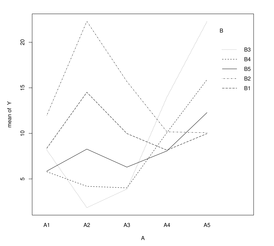
Reading Interaction Plots
Plot \(\overline Y_{ij}\) in function of modalities \((i,j)\)
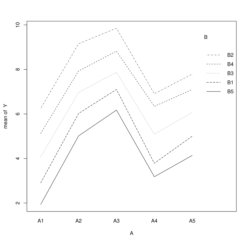
Interaction Plots: Lines Cross
Lines cross in presence of interaction
Interaction plot — drag the cell means
Drag a cell mean (solid = theoretical \(\mu_{ij}\); light dashed = empirical \(\hat Y_{ij}\), with noise). Pick the active cell with the i / j buttons; hover a point to read its value. The interaction term \(\gamma_{ij}\) turns green and \(\to 0\) when the lines are parallel.
Testing Strategy: Interaction First
We want to test for the presence of an interaction:
\[H_0^{(AB)}: \gamma_{ij} = 0 \text{ for all } i, j\]
If we conclude \(H_0^{(AB)}\) (accept the null hypothesis), we then want to test the marginal effects:
\[H_0^{(A)}: \alpha_i = 0 \text{ for all } i \and H_0^{(B)}: \beta_j = 0 \text{ for all } j\]
When the Interaction Is Significant
\[H_0^{(AB)}: \gamma_{ij} = 0 \text{ for all } i, j\]
Warning
If we reject \(H_0^{(AB)}\), it makes no sense to test whether A or B have an effect: they have one through their interaction.
These tests reduce to constraint tests in the regression model.
Balanced Design Analysis of Variance
We assume that “the design is balanced”: this means that \(N_{ij}:=N\) does not depend on \(i\) or \(j\). (Otherwise, everything becomes complicated).
In this case, we have the analysis of variance formula:
ANOVA Formula
\[S_T^2 = S_A^2 + S_B^2 + S_{AB}^2 + S_R^2\]
\(S_T^2 = \sum_{k=1}^{n} (Y_{k} - \overline{Y})^2\): total sum of squares
\(S_A^2 = \sum_{i=1}^{I} \sum_{j=1}^{J} N_{ij} (\overline{Y}_{i.} - \overline{Y})^2\): \(S^2_{between}\) in the case of one-factor ANOVA where the factor is \(A\)
\(S_B^2 = \sum_{i=1}^{I} \sum_{j=1}^{J} N_{ij} (\overline{Y}_{.j} - \overline{Y})^2\): \(S^2_{between}\) in the case of one-factor ANOVA where the factor is \(B\)
\(S_{AB}^2 = \sum_{i=1}^{I} \sum_{j=1}^{J} N_{ij} (\overline{Y}_{ij} - \overline{Y}_{i.} - \overline{Y}_{.j} + \overline{Y})^2\) quantifies the interaction
\(S_R^2 = \sum_{i=1}^{I} \sum_{j=1}^{J} \sum_{k=1}^{N_{ij}} (Y_{k} - \overline{Y}_{ij})^2\1\{X^{(1)}_k=A_i \and X^{(2)}_k=B_j\}\): \(S_{within}\) in one-factor ANOVA
Testing the Interaction: Constraint Test
For testing the interaction, \(H_0^{(AB)}: \gamma_{ij} = 0\) for all \(i, j\)
We use the linear constraint test statistic \(F = \frac{n-p}{q} \frac{(SSR_c - SSR)}{SSR}\)
where \(SSR_c\) corresponds to the sum of squares of the residuals in the space \(\gamma_{ij}=0\) for all \((i,j)\).
Testing the Interaction: F Statistic
\[F^{(AB)} = \frac{S_{AB}^2/\big((I-1)(J-1)\big)}{S_R^2/(n-IJ)}\]
When \(\varepsilon \sim \mathcal N(0, \sigma^2 I_n)\), \(F^{(AB)} \sim \mathcal F((I-1)(J-1), n-IJ)\)
Testing the Effect of A
For testing the main effect of \(A\), \(H_0^{(A)}: \alpha_i = 0\) for all \(i\):
We use \(F = \frac{n-p}{q} \frac{(SSR_c - SSR)}{SSR}\)
where \(SSR_c\) corresponds to the sum of squares of the residuals in the space \(\alpha_i=0\) for all \(i\).
\[F^{(A)} = \frac{S_A^2/(I-1)}{S_R^2/(n-IJ)}\]
When \(\varepsilon \sim \mathcal{N}(0, \sigma^2 I_n)\), \(F^{(A)} \sim \mathcal{F}(I-1, n-IJ)\)
Testing the Effect of B
For testing the main effect of \(B\), \(H_0^{(B)}: \beta_j = 0\) for all \(j\):
We use \(F = \frac{n-p}{q} \frac{(SSR_c - SSR)}{SSR}\)
where \(SSR_c\) corresponds to the sum of squares of the residuals in the space \(\beta_j=0\) for all \(j\).
\[F^{(B)} = \frac{S_B^2/(J-1)}{S_R^2/(n-IJ)}\]
When \(\varepsilon \sim \mathcal{N}(0, \sigma^2 I_n)\), \(F^{(B)} \sim \mathcal{F}(J-1, n-IJ)\)
R outputs
In software, these tests are summarized in a table as shown below.
In R: anova(lm(Y ~ A*B))
| Source | df | Sum Sq | Mean Sq | F value | Pr(>F) |
|---|---|---|---|---|---|
| \(A\) | \(I-1\) | \(S_A^2\) | \(S_A^2/(I-1)\) | \(F^{(A)}\) | … |
| \(B\) | \(J-1\) | \(S_B^2\) | \(S_B^2/(J-1)\) | \(F^{(B)}\) | … |
| \(A:B\) | \((I-1)(J-1)\) | \(S_{AB}^2\) | \(S_{AB}^2/((I-1)(J-1))\) | \(F^{(AB)}\) | … |
| Residuals | \(n-IJ\) | \(S_R^2\) | \(S_R^2/(n-IJ)\) |
Two-Way ANOVA in Practice
Assumptions
Fisher tests are based on the assumption \(\varepsilon \sim N(0, \sigma^2 I_n)\)
- Normality is not critical, but homoscedasticity is
- We can test equality of variances in each modality of A (or B), or in each crossed modality if the \(n_{ij}\) are sufficiently large
- This can be done with Levene’s test or Bartlett’s test
Practical Procedure
Test equality of variances
Form the ANOVA table (independent of chosen constraints)
If the \(AB\) interaction is significant: don’t change anything
If the interaction is not significant: analyze the marginal effects of A and B
- If they are significant: the model is additive:
lm(Y ~ A + B) - Otherwise: we can remove \(A\) (or \(B\)) from the model
Post-Hoc Analysis
Once effects are identified: perform post-hoc analysis by examining differences between (crossed) modalities more closely, using Tukey’s test as in one-factor ANOVA
Beyond Two Factors
Principle and Limits
We seek to explain \(Y\) using \(k\) qualitative variables \(A=X^{(1)}\), \(B=X^{(2)}\), \(C=X^{(3)}\), …
We can assume that \(\E[Y_k]\) depends on each factor and their interactions:
- Two-way interactions: \(AB\), \(BC\), \(AC\), etc.
- Three-way interactions: \(ABC\), etc.
- Higher-order interactions: and potentially more
Warning
This results in \(2^k - 1\) possible effects for \(k\) factors.
Testing Approach
Each effect can be tested using linear constraint tests. However, this approach presents several challenges:
- Multiple testing burden: Too many tests to perform
- Sample size limitations: Risk of insufficient sample sizes in each crossed modality
In practice, choices are made to include only a limited number of effects and interactions in the analysis.
Analysis of Covariance (ANCOVA)
Model Components
Most general situation: we seek to explain Y using both quantitative and qualitative variables.
Quantitative variable effects: Through each regression coefficient \(\beta_j\) associated with each variable
Factor effects and interactions: As in ANOVA analysis
- Main effects of factors (quali. var.)
- Interactions between factors
Mixed interactions: Effects of interactions between factors and quantitative variables
Example of Mixed Interaction
- \(A \in \{\text{Labrador}, \text{Chihuahua}\}\)
- \(X^{(1)}\): size of the dog
- There is clearly a mixed interaction between factor \(A\) and \(X^{(1)}\)!
Statistical Testing
Each effect can be tested using a Fisher test.
Obviously, choices must be made regarding which effects and interactions to include in the model.
ANCOVA in R: Quantitative & Qualitative Variables
Model Without Interaction
\(Y\): quantitative response variable
\(X\): quantitative variable,
\(Z\): factor with \(I\) modalities \(\{A_1, \dots, A_I\}\)
lm(Y~X+Z) estimates the model without interaction, where, for each individual \(k = 1, \ldots, n\):
\[Y_k = m + \beta X_k + \sum_{i=2}^{I} \alpha_i \mathbf{1}\{Z_k=A_i\} + \varepsilon_k\]
Constraint \(\alpha_1 = 0\) is adopted to make the model identifiable.
Model With Interaction
lm(Y~X+A+X:A) or lm(Y~X*A) estimates the model with interaction:
\[ \begin{aligned} Y_k &= m + \beta X_k + \sum_{i=2}^{I} \beta_i X_k \mathbf{1}\{Z_k=A_i\} \\ &+ \sum_{i=2}^{I} \alpha_i \mathbf{1}\{Z_k=A_i\} + \varepsilon_k \end{aligned} \]
Key Insight: In the interaction model, the coefficient \(\beta\) associated with \(X\) varies according to the modality \(A_i\).