Counting Models
Log-Linear Poisson Model
\(\newcommand{\VS}{\quad \mathrm{VS} \quad}\) \(\newcommand{\and}{\quad \mathrm{and} \quad}\) \(\newcommand{\E}{\mathbb E}\) \(\newcommand{\P}{\mathbb P}\) \(\newcommand{\Var}{\mathbb V}\) \(\newcommand{\Cov}{\mathrm{Cov}}\) \(\newcommand{\1}{\mathbf 1}\)
Model Assumption
We assume that
\[Y_i|X_i=x_i \sim P(\lambda_\beta(x_i))\quad \text{with} \quad \lambda_\beta(x) = \exp(x^T \beta)\]
with \(\lambda_\beta(x) = \exp(x^T \beta)\).
In particular, \(\mathbb E[Y_i|X_i=x_i] = \lambda_\beta(x)\)
Warning
\(Y|X\) follows a Poisson distribution but not \(Y\) if \(X\) is random!
(We can only say that it is a mixture of Poisson)
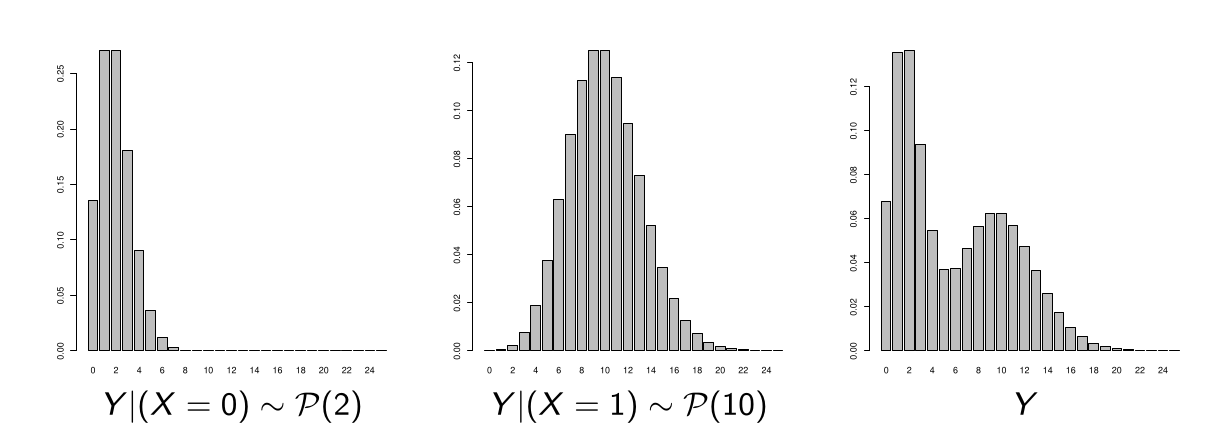
Illustration
Example: binary regressor \(X\) (with as many \(X = 0\) as \(X = 1\))
\(Y|(X = 0) \sim P(2) \and Y|(X = 1) \sim P(10)\)
Rate Ratio
There is no notion of OR since we are not estimating a probability (or a probability ratio) but an expectation.
The equivalent notion here is the rate ratio (RR), \(\lambda(x)\) being seen as an average rate of occurrence of \(Y\).
For two characteristics \(x_1\) and \(x_2\), the rate ratio is simply:
\[RR(x_1, x_2) = \frac{\lambda_\beta(x_1)}{\lambda_\beta(x_2)} = \exp((x_1 - x_2)^T \beta)\]
Particular Cases for Rate Ratio
Single Regressor Difference: If \(x_1\) and \(x_2\) differ only by regressor \(j\):
\(RR(x_1, x_2) = \exp((x_{1j} - x_{2j})\beta_j)\)
Binary regressor: (\(x_{1j} = 1\) and \(x_{2j} = 0\)): \(RR_j = e^{\beta_j}\).
Log-Likelihood
\[P(Y = k|X = x) = e^{-\lambda_\beta(x)} \frac{\lambda_\beta(x)^k}{k!}\]
Thus the sample likelihood equals \(\prod_{i=1}^n e^{-\lambda_\beta(x_i)} \frac{\lambda_\beta(x_i)^{y_i}}{y_i!}\)
Since \(\lambda_\beta(x) = \exp(x^T \beta)\), the log-likelihood therefore equals
\[L = \sum_{i=1}^n \left[y_i x_i^T \beta - e^{x_i^T \beta} - \ln(y_i!)\right]\]
Estimation of β by MLE
By setting the gradient with respect to \(\beta\) to zero, we find that the MLE \(\hat{\beta}\) must verify:
\[\sum_{i=1}^n y_i x_i = \sum_{i=1}^n \lambda_{\hat{\beta}}(x_i) x_i\]
This is a system with \(p\) unknowns (recall that \(x_i \in \mathbb R^p\)) that we solve numerically.
Properties of β̂
Under regularity conditions, when \(n \to \infty\):
\[\hat{\beta} \sim N(\beta, (X^T W_{\hat{\beta}} X)^{-1})\]
where \(W_{\hat{\beta}} = \text{diag}(\lambda_{\hat{\beta}}(x_1), \ldots, \lambda_{\hat{\beta}}(x_n))\).
We can therefore perform Wald significance tests.
Validation: Deviance
The saturated model (one parameter per different observation) leads to
\[\hat{\lambda}(x) = \frac{y_x}{n_x}\]
- \(y_x = \sum_{i:x_i=x} y_i\) is the total number of \(Y\) observed for characteristic \(x\) on the sample
- \(n_x = \sum_{i:x_i=x} 1\) is the number of times \(x\) was observed.
Saturated Log-Likelihood
The log-likelihood of the saturated model therefore equals:
\[L_{\text{sat}} = \sum_x \left[y_x \ln\left(\frac{y_x}{n_x}\right) - y_x\right] - \text{cste}\]
where \(\text{cste} = \sum_{i=1}^n \ln(y_i!)\).
Deviance Formula
Thus the deviance equals
\[D = 2(L_{\text{sat}} - L_{\text{mod}}) = 2\sum_x y_x \ln\left(\frac{y_x}{n_x \lambda_{\hat{\beta}}(x)}\right) - (y_x - n_x \lambda_{\hat{\beta}}(x))\]
If a constant is in the model (one coordinate of \(x\) equals \(1\)), we have from the likelihood equations \(\sum_x y_x = \sum_x n_x \lambda_{\hat{\beta}}(x)\) and then
\[D = 2\sum_x y_x \ln\left(\frac{y_x}{\hat{y}_x}\right)\]
where \(\hat{y}_x = n_x \lambda_{\hat{\beta}}(x)\) are the expected theoretical counts.
Validation: Deviance Test
As in logistic regression, we can compare two nested models by a deviance test (or likelihood ratio test)
If model 2 has \(q\) fewer parameters compared to model 1, we have under \(H_0\): “the \(q\) coefficients in question are zero”:
\[D_2 - D_1 = 2(L_1 - L_2) \xrightarrow{L} \chi^2_q\]
Rejection region at level \(\alpha\):
\[\text{CR}_\alpha = \{D_2 - D_1 > \chi^2_q(1-\alpha)\}\]
Global Significance Test
The global significance test corresponds to the case where model 2 contains only the constant.
In this case \(D_2 = D_0\) and \(q = p - 1\).
Validation: Graphical Inspection
Plot the predicted counts \(\hat{y}_x = n_x \lambda_{\hat{\beta}}(x)\) against the observed counts \(y_x\).
Warning
the predicted counts \(\hat{y}_x\) represent the expectation of the expected counts given \(x\).
It is therefore normal that the observed counts \(y_x\) are dispersed around the \(\hat{y}_x\)
It is appropriate to have sufficiently large “classes” \(x\) (\(n_x > 5\)) for the graph to be relevant.
Alternative Graphical Validation
Idea: empirical distribution of \(Y\) VS its predicted distribution.
The empirical distribution of \(Y\) is simply given by
\(p_k = \frac{1}{n}\sum_{i=1}^n \mathbf{1}_{y_i = k}, \quad k \in \mathbb{N}\)
While its predicted distribution is given by
\(\hat{p}_k = \frac{1}{n}\sum_{i=1}^n \hat{P}(Y = k|X = x_i), \quad k \in \mathbb{N}\)
where \(\hat{P}(Y = k|X = x_i)\) is the poisson distribution \(\mathcal P(\lambda_{\hat{\beta}}(x_i))\), i.e., \(\hat{P}(Y = k|X = x_i) = \frac{\lambda_{\hat{\beta}}(x_i)^k e^{-\lambda_{\hat{\beta}}(x_i)}}{k!}\)
Example: Number of Plant Species
Number of plant species recorded on a plot according to soil pH (Neutral, Acidic or Basic) and biomass collected.
| Species | pH | Biomass |
|---|---|---|
| 14 | low | 3.538 |
| 31 | mid | 0.740 |
| 36 | high | 7.242 |
| 20 | mid | 3.216 |
| … | … | … |
We want to model \(Y =\) “Species” as a function of pH and Biomass.
Example: R output
| Coefficient | Estimate | Std. Error | z value | Pr(> | z |
|---|---|---|---|---|---|
| (Intercept) | 3.84894 | 0.05281 | 72.885 | < 2e-16 | *** |
| pHlow | -1.13639 | 0.06720 | -16.910 | < 2e-16 | *** |
| pHmid | -0.44516 | 0.05486 | -8.114 | 4.88e-16 | *** |
| Biomass | -0.12756 | 0.01014 | -12.579 | < 2e-16 | *** |
Signif. codes: 0 ‘’ 0.001 ’’ 0.01 ’’ 0.05 ‘.’ 0.1 ’ ’ 1
(Dispersion parameter for poisson family taken to be 1)
Null deviance: 452.346
Residual deviance: 99.242
AIC: 526.43
Example: Number of Plant Species
Thus, the average number of species, given pH and Biomass, is estimated as
\(\lambda_{\hat{\beta}}(\text{pH}, \text{Biomass}) = \exp(3.85 - 1.14 \mathbf{1}_{\text{pH=low}} - 0.46 \mathbf{1}_{\text{pH=mid}} - 0.13 \text{Biomass})\)
Rate Ratio for low pH (acidic) compared to high pH (basic):
\(RR(\text{acidic}, \text{basic}) = \exp(-1.14) = 0.32\)
On average, there are therefore about 3 times fewer species in acidic soil than in basic soil.
Example: Interraction Ph-Biomass
We can try to introduce an interaction between pH and Biomass
| Coefficient | Estimate | Std. Error | z value | Pr(> | z |
|---|---|---|---|---|---|
| (Intercept) | 3.76812 | 0.06153 | 61.240 | < 2e-16 | *** |
| pHlow | -0.81557 | 0.10284 | -7.931 | 2.18e-15 | *** |
| pHmid | -0.33146 | 0.09217 | -3.596 | 0.000323 | *** |
| Biomass | -0.10713 | 0.01249 | -8.577 | < 2e-16 | *** |
| pHlow:Biomass | -0.15503 | 0.04003 | -3.873 | 0.000108 | *** |
| pHmid:Biomass | -0.03189 | 0.02308 | -1.382 | 0.166954 |
Signif. codes: 0 ‘’ 0.001 ’’ 0.01 ’’ 0.05 ‘.’ 0.1 ’ ’ 1
(Dispersion parameter for poisson family taken to be 1)
Null deviance: 452.346
Residual deviance: 83.201
AIC: 514.39
Example: Model Comparison
The model with interaction seems preferable (via AIC and deviance test).
The average number of species, given pH and Biomass, is this time:
\[\begin{aligned} \lambda_{\hat{\beta}}(\text{pH}, \text{Bm}) &= \exp(3.77 - 0.82 \mathbf{1}_{\text{pH=low}} - 0.33 \mathbf{1}_{\text{pH=mid}}) \\ &- 0.11\text{Bm} - 0.16\text{Bm}\mathbf{1}_{\text{pH=low}} - 0.032\text{Bm}\mathbf{1}_{\text{pH=mid}} \end{aligned}\]
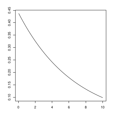
Example: Bm-dependent RR
The Rate Ratio for low pH (acidic) compared to high pH (basic) depends on Biomass and equals:
\(RR(\text{acidic}, \text{basic}) = \exp(-0.82 - 0.16\text{Bm})\)
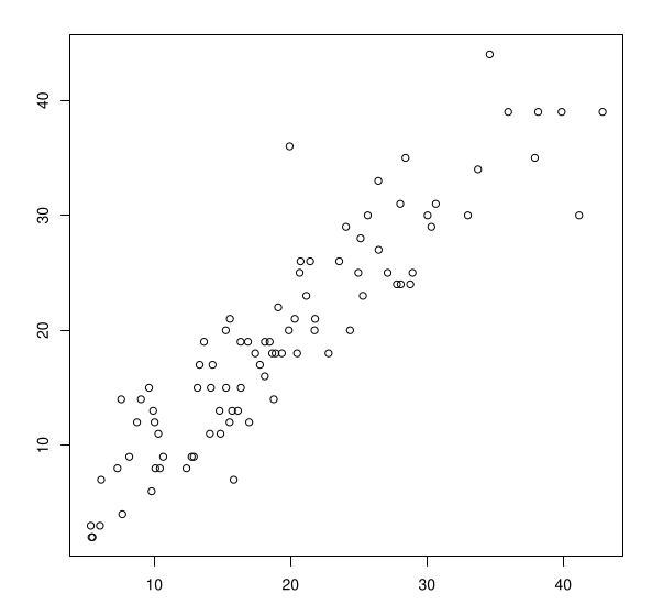
Example: Predicted vs Observed Counts
Predicted mean counts \(\hat{y}_i = \lambda_{\hat{\beta}}(\text{pH}_i, \text{Biomass}_i)\) as a function of observed counts \(y_i\).
Model Predictions by pH
Lines: predicted mean counts by pH as a function of biomass
Points: observed counts by pH as a function of biomass
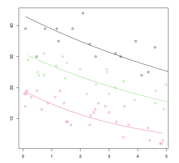
Black: pH=basic; Green: pH=neutral; Red: pH=acidic
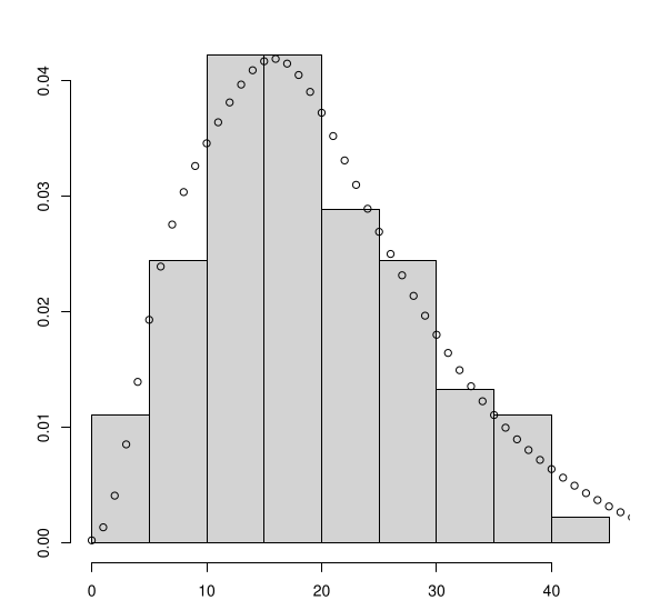
Predicted Distribution
Histogram: empirical distribution
Points: predicted distribution
Overdispersion
Model Limitations
When we model \(Y|(X = x) \sim \mathcal P(\lambda(x))\), we have
\[\E(Y|X = x) = \lambda(x)\]
but also
\[\Var(Y|X = x) = \lambda(x)\]
This constraint is a limitation of the Poisson model.
Overdispersion
Some data are overdispersed, in the sense that
\[\Var(Y|X = x) > \E(Y|X = x)\]
More rarely, we can find underdispersed data.
In case of overdispersion, the estimated variance of estimators is underestimated.
How to Detect Overdispersion?
By assuming that \(\Var(Y|X = x) = \phi \E(Y|X = x)\) where \(\phi > 0\), we can estimate \(\phi\) by
\[\hat{\phi} = \frac{1}{n-p} \sum_{i=1}^n \frac{(y_i - \hat{y}_i)^2}{\hat{y}_i}\]
and test if \(\phi = 1\) or not (if \(\phi = 1\), \(\hat{\phi} \sim N(1, 1/n)\) when \(n \to \infty\)).
We can fit a negative binomial model (cf the following), and test if it is better than the Poisson model.
The Quasi-Poisson Model
Estimate \(E(Y|X = x) = \lambda_\beta(x)\) with \(\lambda_\beta(x) = \exp(x^T \beta)\) in the same way as with a Poisson model (same likelihood).
Estimate \(\phi\) as in the previous slide.
Estimate the variance of \(\hat{\beta}\) taking into account \(\hat{\phi}\).
Quasi-Poisson VS Poisson Model
- The estimated coefficients \(\hat{\beta}\) are identical.
- The predictions \(\hat{y}_i = \exp(\lambda_{\hat{\beta}}(x_i))\) are identical.
- Only the estimation of standard errors differ, and therefore possibly the significance of coefficients.
The estimation procedure does not rely on the “true” likelihood (because of \(\phi\)): we therefore do not have access to \(L_{\text{mod}}\).
Example: Plant Species with Quasi Poisson
| Coefficient | Estimate | Std. Error | t value | Pr(> | t |
|---|---|---|---|---|---|
| (Intercept) | 3.76812 | 0.06144 | 61.332 | < 2e-16 | *** |
| pHlow | -0.81557 | 0.10268 | -7.943 | 7.90e-12 | *** |
| pHmid | -0.33146 | 0.09203 | -3.602 | 0.000534 | *** |
| Biomass | -0.10713 | 0.01247 | -8.590 | 3.97e-13 | *** |
| pHlow:Biomass | -0.15503 | 0.03997 | -3.878 | 0.000208 | *** |
| pHmid:Biomass | -0.03189 | 0.02304 | -1.384 | 0.169985 |
Signif. codes: 0 ‘’ 0.001 ’’ 0.01 ’’ 0.05 ‘.’ 0.1 ’ ’ 1
(Dispersion parameter for quasipoisson family taken to be 0.9970074)
Null deviance: 452.346 on 89 degrees of freedom
Residual deviance: 83.201 on 84 degrees of freedom
AIC: NA
Interpretation
\(\hat{\phi} = 0.997 \approx 1\) therefore there was no overdispersion issue
The Residual deviance is incorrect: it’s that of the Poisson model.
Negative Binomial Distribution
Alternative to Poisson: Negative Binomial (NB), which depends on 2 parameters:
- its expectation \(\lambda > 0\)
- the “number of successes” (or size) \(\theta > 0\)
If \(Y \sim NB(\lambda, \theta)\), then for all \(k \in \mathbb{N}\),
\[P(Y = k) = \frac{\Gamma(k + \theta)}{\Gamma(k + 1)\Gamma(\theta)} \left(\frac{\lambda}{\lambda + \theta}\right)^k \left(\frac{\theta}{\lambda + \theta}\right)^\theta\]
Properties of Negative Binomial
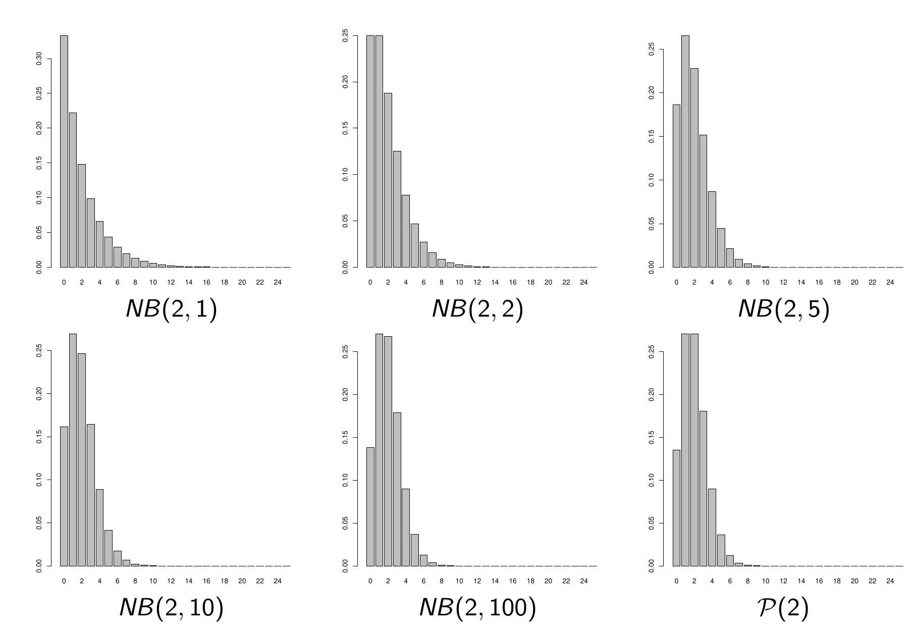
The expectation of \(NB(\lambda, \theta)\) equals \(\lambda\).
The variance of \(NB(\lambda, \theta)\) equals \(\lambda + \lambda^2/\theta\).
This distribution can therefore model overdispersion (but not underdispersion).
If \(\theta \to +\infty\), \(NB(\lambda, \theta) \approx P(\lambda)\).
The Poisson distribution is therefore a special case of the NB distribution.
Illustration of NB
Negative Binomial GLM Model
The negative binomial GLM model assumes that
\[Y|(X = x) \sim NB(\lambda(x), \theta)\]
where as usual \(\lambda(x) = \exp(x^T \beta)\).
Inference an other Tools in NB GLM model
The estimation of \(\beta\) and \(\theta\) is done by maximum likelihood
All usual inference tools are available:
- Wald tests; Deviance; AIC, BIC.
If \(\hat{\theta}\) is large, this is equivalent to the Poisson model.
We can test the interest of the NB model compared to the Poisson model by inspecting \(\hat{\theta}\), or by comparing their AIC and BIC criteria.
Example: Plant Species and NB Model
| Coefficient | Estimate | Std. Error | z value | Pr(> | z |
|---|---|---|---|---|---|
| (Intercept) | 3.76813 | 0.06154 | 61.235 | < 2e-16 | *** |
| pHlow | -0.81557 | 0.10284 | -7.930 | 2.19e-15 | *** |
| pHmid | -0.33146 | 0.09217 | -3.596 | 0.000323 | *** |
| Biomass | -0.10713 | 0.01249 | -8.577 | < 2e-16 | *** |
| pHlow:Biomass | -0.15503 | 0.04003 | -3.873 | 0.000108 | *** |
| pHmid:Biomass | -0.03189 | 0.02308 | -1.382 | 0.166978 |
Signif. codes: 0 ‘’ 0.001 ’’ 0.01 ’’ 0.05 ‘.’ 0.1 ’ ’ 1
(Dispersion parameter for Negative Binomial(212058.3) family taken to be 1)
Null deviance: 452.307 on 89 degrees of freedom
Residual deviance: 83.194 on 84 degrees of freedom
AIC: 516.39
\(\hat{\theta} = 212058.3\) therefore the model is equivalent to the Poisson model.
This is confirmed via the AIC.
Zero-inflated Models
The Problem
When \(Y\) is a count variable, it is not uncommon for \(Y = 0\) to appear very often in the sample.
Example 1: \(Y\): amount of rain (in mm) that fell each day.
Example 2: \(Y\): amount of alcohol (in glasses) consumed each week.
Model Inadequacy
A Poisson or Negative Binomial model is not adapted.
Generally two “populations” that explain this phenomenon:
- one for which \(Y = 0\) systematically
- one for which \(Y \geq 0\) (or \(Y > 0\))
We can consider two modelings in this spirit:
- The zero-inflated model (\(Y = 0\) versus \(Y \geq 0\))
- The Hurdle model (\(Y = 0\) versus \(Y > 0\))
We present below the zero-inflated model.
ZIP Model Definition
The ZIP (Zero-Inflated Poisson) model assumes that
\[Y|(X = x) = \begin{cases} 0 & \text{with probability } q(x) \\ P(\lambda(x)) & \text{with probability } 1 - q(x) \end{cases}\]
where
\[\lambda(x) = \exp(x^T \beta) \quad \text{and} \quad q(x) = \text{logit}^{-1}(x^T \gamma)\]
Two Mixed Populations
Thus two populations mix:
- For one, \(Y\) is always \(0\). For the other, \(Y \in \mathbb{N}\).
- A logistic model explains membership to one or the other population.
- A Poisson log-linear model is used for the second.
Probability Distribution
With this model, we therefore have
\(P(Y = 0|X = x) = q_\gamma(x) + (1 - q_\gamma(x))e^{-\lambda_\beta(x)}\)
\(P(Y = k|X = x) = (1 - q_\gamma(x))e^{-\lambda_\beta(x)} \frac{\lambda_\beta(x)^k}{k!}\)
where \(\lambda_\beta(x) = \exp(x^T \beta)\) and \(q_\gamma(x) = \text{logit}^{-1}(x^T \gamma)\).
We deduce
\(E(Y|X = x) = (1 - q_\gamma(x))\lambda_\beta(x)\)
Inference
For inference:
- We can write the log-likelihood as a function of \(\beta\) and \(\gamma\)
- We obtain estimators by maximum likelihood
- And we have access to usual inference tools
Under R: zeroinfl function from the pscl package.
ZINB Model Definition
Similarly, the ZINB (Zero-Inflated Negative Binomial) model is
\[Y|(X = x) = \begin{cases} 0 & \text{with probability } q(x) \\ NB(\lambda(x), \theta) & \text{with probability } 1 - q(x) \end{cases}\]
where \(\theta > 0\) and
\(\lambda(x) = \exp(x^T \beta) \quad \text{and} \quad q(x) = \text{logit}^{-1}(x^T \gamma)\)
Under R: zeroinfl function with the option dist="negbin".
Example: Horseshoe Crabs
Number of male satellites on female horseshoe crabs.
We want to model the number of satellites (satell) as a function of the weight of the horseshoe crab (weight) and its color (color, from 1 to 4, ≈ age).
Example: Poisson log-linear Model :
| Coefficient | Estimate | Std. Error | z value | Pr(> | z |
|---|---|---|---|---|---|
| (Intercept) | 0.08855 | 0.25443 | 0.348 | 0.72783 | |
| weight | 0.54588 | 0.06749 | 8.088 | 6.05e-16 | *** |
| color | -0.17282 | 0.06155 | -2.808 | 0.00499 | ** |
Signif. codes: 0 ‘’ 0.001 ’’ 0.01 ’’ 0.05 ‘.’ 0.1 ’ ’ 1
(Dispersion parameter for poisson family taken to be 1)
Null deviance: 632.79 on 172 degrees of freedom
Residual deviance: 552.79 on 170 degrees of freedom
AIC: 914.09
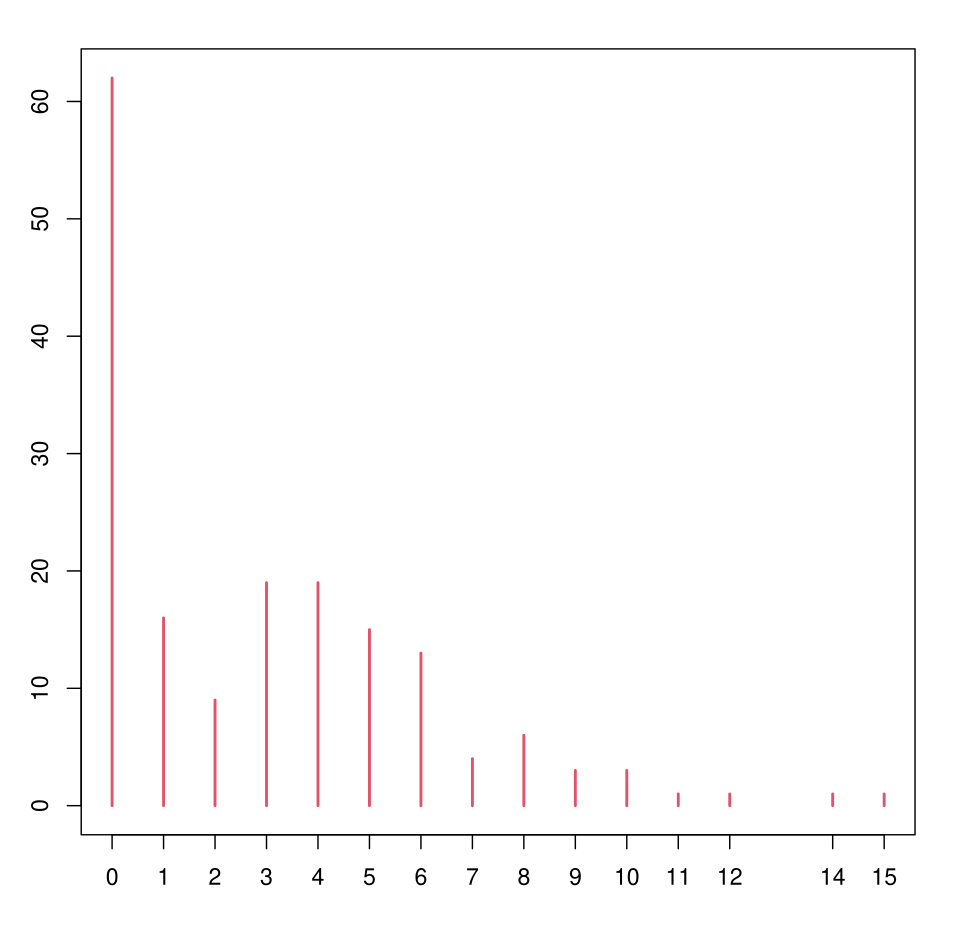
The model is significant but the fit is poor (the deviance is very high)
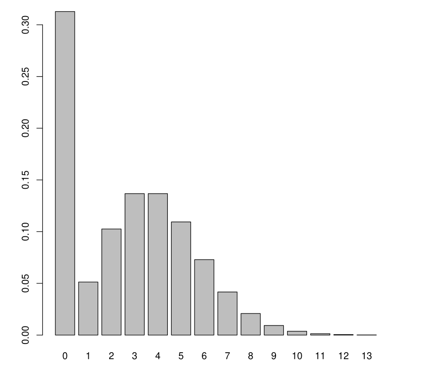
Example: Log-Linear Poisson
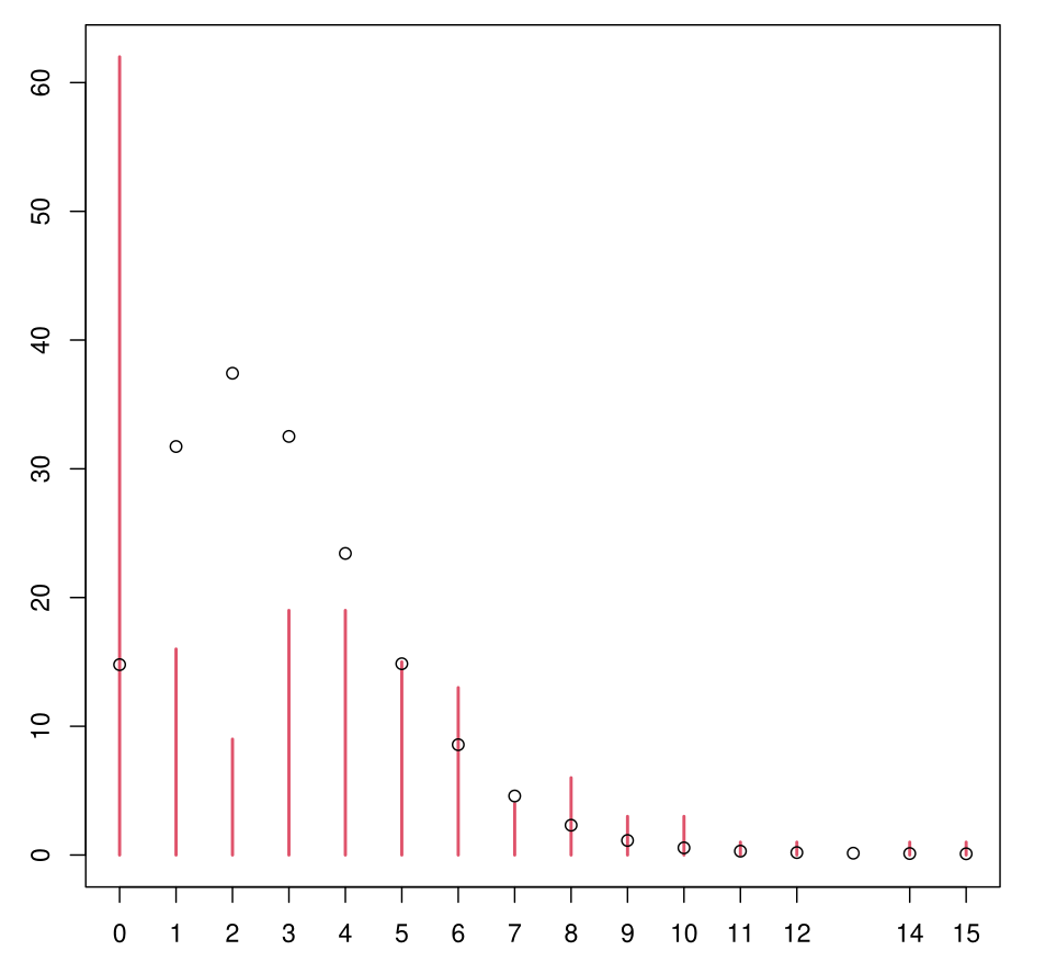
- In red: empirical distribution of satell on the sample
- Points: predicted distribution
Example: NB Model
| Coefficient | Estimate | Std. Error | z value | Pr(> | z |
|---|---|---|---|---|---|
| (Intercept) | -0.3220 | 0.5540 | -0.581 | 0.561 | |
| weight | 0.7072 | 0.1612 | 4.387 | 1.15e-05 | *** |
| color | -0.1734 | 0.1199 | -1.445 | 0.148 |
Signif. codes: 0 ‘’ 0.001 ’’ 0.01 ’’ 0.05 ‘.’ 0.1 ’ ’ 1
(Dispersion parameter for Negative Binomial(0.9555) family taken to be 1)
Null deviance: 219.50 on 172 degrees of freedom
Residual deviance: 196.64 on 170 degrees of freedom
AIC: 754.45
It’s better… (by the way: color doesn’t seem significant)
Example: NB Model
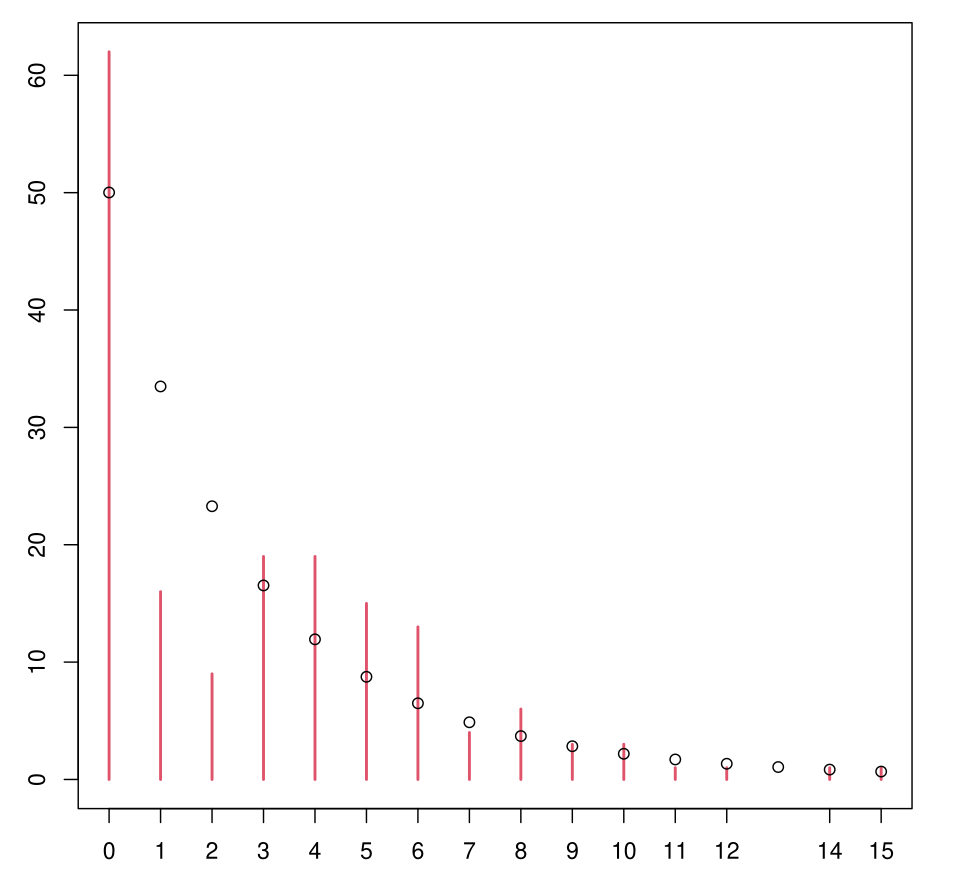
Still not very satisfactory.
Example: ZIP Model
Count model coefficients (poisson with log link):
| Coefficient | Estimate | Std. Error | z value | Pr(> | z |
|---|---|---|---|---|---|
| (Intercept) | 1.00152 | 0.20793 | 4.817 | 1.46e-06 | *** |
| weight | 0.19020 | 0.07572 | 2.512 | 0.012 | * |
Zero-inflation model coefficients (binomial with logit link):
| Coefficient | Estimate | Std. Error | z value | Pr(> | z |
|---|---|---|---|---|---|
| (Intercept) | 1.9621 | 1.1448 | 1.714 | 0.0866 | . |
| weight | -1.6630 | 0.3943 | -4.218 | 2.47e-05 | *** |
| color | 0.5329 | 0.2305 | 2.312 | 0.0208 | * |
Signif. codes: 0 ‘’ 0.001 ’’ 0.01 ’’ 0.05 ‘.’ 0.1 ’ ’ 1
Number of iterations in BFGS optimization: 9
Log-likelihood: -360.8 on 5 Df
Example: ZIP Model
We see the estimation result explaining the mixture of the two “populations” forming the model.
First population: Poisson log-linear model with expectation \(\lambda\) where \(\lambda(\text{weight}) = \exp(1 + 0.19 \times \text{weight})\)
Second population is \(0\). The probability \(q\) of belonging to the second one is
\(q(\text{wgt}, \text{col}) = \text{logit}^{-1}(1.96 - 1.66 \times \text{wgt} + 0.53 \times \text{col})\)
Example: ZIP Model
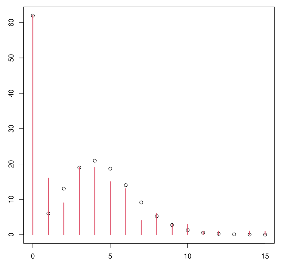
Much more convincing.
Example: ZINB Model
Count model coefficients (negbin with log link):
| Coefficient | Estimate | Std. Error | z value | Pr(> | z |
|---|---|---|---|---|---|
| (Intercept) | 0.8961 | 0.3070 | 2.919 | 0.00351 | ** |
| weight | 0.2169 | 0.1125 | 1.928 | 0.05383 | . |
| Log(theta) | 1.5802 | 0.3574 | 4.422 | 9.79e-06 | *** |
Zero-inflation model coefficients (binomial with logit link):
| Coefficient | Estimate | Std. Error | z value | Pr(> | z |
|---|---|---|---|---|---|
| (Intercept) | 1.8663 | 1.2415 | 1.503 | 0.133 | |
| weight | -1.7531 | 0.4429 | -3.958 | 7.55e-05 | *** |
| color | 0.5985 | 0.2572 | 2.326 | 0.020 | * |
Signif. codes: 0 ‘’ 0.001 ’’ 0.01 ’’ 0.05 ‘.’ 0.1 ’ ’ 1
Theta = 4.8558
Number of iterations in BFGS optimization: 11
Log-likelihood: -349.9 on 6 Df
Example: ZINB Model
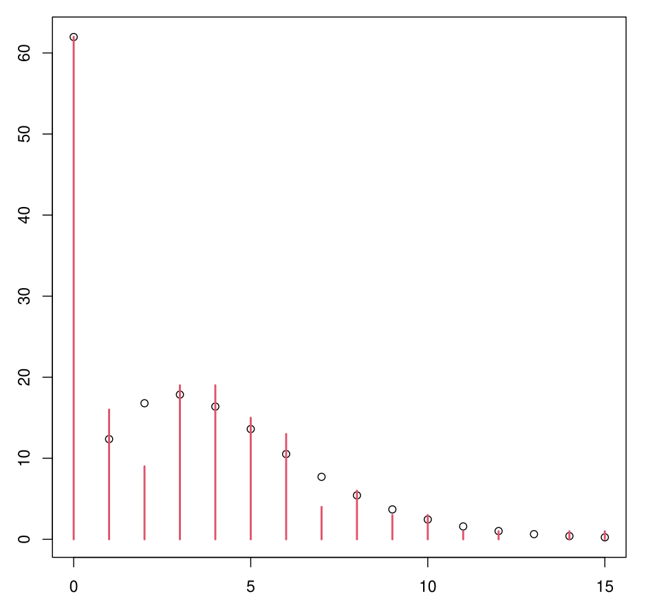
ZINB Model Interpretation
The output is read in the same way as for the ZIP model
There is the parameter \(\theta\) in addition, from the NB distribution
\(\theta\) is not “infinite”: the model therefore does not reduce to the ZIP model.
A deviance test shows that ZINB is preferable to ZIP
This is also confirmed by the AIC and BIC criteria.
Example: Conclusion
A portion of horseshoe crabs (the smallest and oldest) have no male satellites.
The probability of belonging to this population is estimated at
\(q(\text{wht}, \text{col}) = \text{logit}^{-1}(1.87 - 1.75 \times \text{wht} + 0.60 \times \text{col})\)
For the other portion of horseshoe crabs, they have on average more satellites the larger they are. This average is estimated at
\(\lambda(\text{wht}) = \exp(0.90 + 0.22 \times \text{wht})\)
Distribution cna be modeled as \(NB(\lambda(\text{wht}), \theta)\) where \(\theta = 4.86\).